Recommender System: Part 1 - Building The Model

Objective

In part 1 of this series, I will demonstrate how to build a collaborative filtering model in python. Training, optimizing, and analyzing the model will follow in subsequent posts.

Background

Data

The data I’ll be using comes from boardgamegeek.com. The raw data has userID, gameID, and ratings columns as in the sample below.

Table 1 | Raw data

userID	gameID	rating
83	39938	7.0
83	34219	7.0
83	24068	7.0
83	70149	8.0
83	43015	9.0

Figure 1 | Ratings Distribution

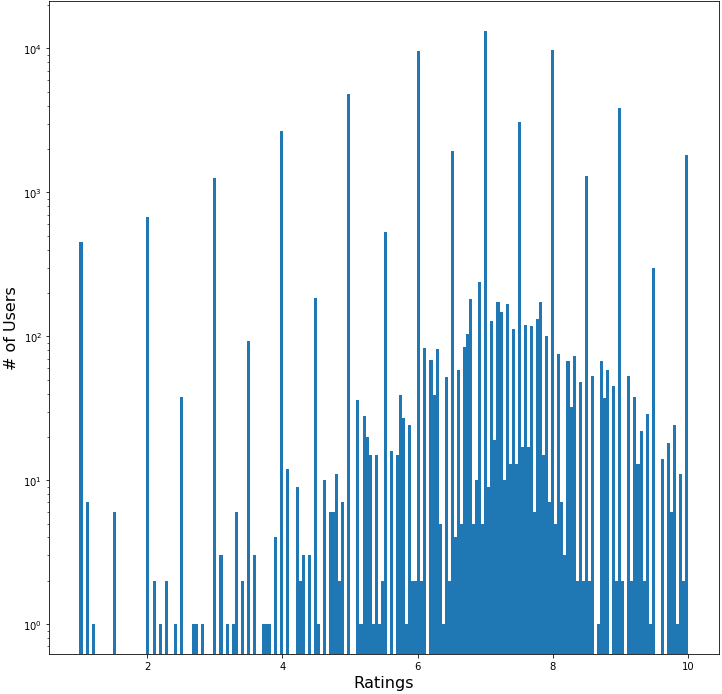
Figure 1 shows the distribution of all user ratings on a semilog plot. The median rating is 7.0. The ratings are clearly quantized at integer and half integer levels. A closer examination reveals further quantized levels at every quarter rating. Below the quarter interval the ratings distribution becomes more continuous.

The Model

The specific type of collaborative filtering model I want to build is commonly referred to as model based, as opposed to content based. The goal is for the model to find underlying features of the data that make good predictors of user ratings for a given game. This is sort of a black box approach because we don’t actually know what these underlying features are. An intuitive assumption is to think of these features as common properties we would associate with board games such as genre, number of players, recommended age, average length of game, etc. If a user is asked to rate a game they’ve never played before, it’s natural to think these properties would play an important role in the user’s rating.

Figure 2 | Matrix Implementation

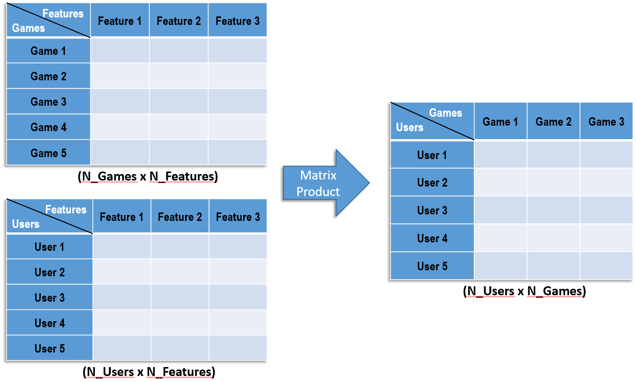
Implementation of the model in python is best optimized using matrix algebra which greatly speeds up calculations that must be performed iteratively. The matrix implementation is illustrated in Figure 2. The data is described by a users matrix and a games matrix. These matrices have a common dimension N_features. These are the features that the model will learn and each individual user or game will be described by a vector of these features. The number of features is a model parameter that we define and tune like the number of neurons in neural network models. To generate a prediction matrix of all users’ predictions on all games, we perform a matrix multiplication as illustrated above.

Code Block 1 | Importing Dependencies

import pandas as pd
import numpy as np
from scipy.optimize import fmin_cg
import cofi

To build this model, we will be using the pandas, numpy, and scipy libraries. The fourth import is a python module I wrote that contains several functions to make running the model more convenient. From the scipy library, we will be using the fmin_cg optimization function. This function requires certain inputs in specific formats which is the nature of the functions written in the cofi module. I will explain these functions as we use them.

Table 2 | Sparse Matrix

userID/gameID	3	5	10	11	12
83	NaN	NaN	NaN	NaN	8.0
119	7.0	7.0	NaN	8.0	NaN
144	NaN	NaN	NaN	7.0	NaN
156	7.5	6.5	NaN	7.0	8.0
186	7.0	NaN	NaN	NaN	8.0

The first step to building the model is to get the data into the right form. We start by pivoting the original data table so that it looks like the sparse matrix in Table 2. This will make comparing predictions easy since we can conveniently use matrix algebra to compute all rating errors in a single line of code. Once we have the sparse matrix, we need to split the data into training and cross-validation (CV) data sets.

Code Block 2 | Generating X_train & X_cv

# Remove a random 20% of the original data for cross-validation
X_cv = data.sample(frac=0.2)

# Blank the corresponding data in the training set.
X_train = data.copy()
X_train.loc[X_cv.index, 'rating'] = np.nan

X_train = X_train.pivot(index='user', columns='game', values='rating')
X_cv = X_cv.pivot(index='user', columns='game', values='rating')

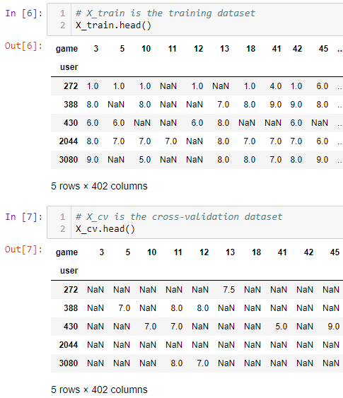
20% of the data is reserved for cross-validation while 80% of the available data will be used for training. In pandas, this is easily done using the .sample(frac=0.2) method where the frac argument indicates we want to sample 20%. The corresponding values in the original dataframe is then blanked to form the training data set (Figure 3). This produces two dataframes, X_train and X_cv:

Figure 3 | X_train & X_cv

In order to use fmin_cg, we will have to provide the following 4 inputs:

1. f(x)	Objective function - This is the function we are trying to optimize.

2. x0	Initial guess - Initial values for an optimal input x.

3. f’(x)

   Gradient of objective function.

4. args	Optional arguments.

Code Block 3 | get_args()

def get_args(X, N_features, Lambda):
    X = np.array(X)
    mu = np.nanmean(X, axis=0)
    Y = X - mu # (N_users x N_games)

    N_users = X.shape[0]
    N_games = X.shape[1]

    # Initialize two random matrices to make our initial predictions
    X_init = np.random.rand(N_games, N_features) - 0.5
    Theta_init = np.random.rand(N_users, N_features) - 0.5

    args = (X_init, Y, Theta_init, Lambda, N_users, N_games, N_features, mu)

    return args

The first function we’ll be using is called get_args() and it takes in 3 arguments.

1. X	a dataframe assumed to be in the form of N_users x N_games (see Figure 3)

2. N_features

   the number of features to use

3. Lambda

   the regularization parameter

The function returns a tuple of 8 parameters that will be fed into fmin_cg as optional parameters. Fmin_cg uses optional parameters to define additional variables needed by the objective and gradient functions. This is exactly what we need since we want to be able to manipulate some of these variables like the regularization parameter and N_features when optimizing the model in the future.

The outputs of the function are:

1. X_init

   the initial guess of the N_games x N_features matrix. (matrix)

2. Y	the actual ratings matrix that we’ve subtracted the mean rating for each game from. This centers each game’s ratings distribution around the same value. The means are added back to the model’s output to generate final predictions. (matrix)

3. Theta_init

   the intial guess of N_users x N_features matrix (matrix)

4. Lambda

   the regularization parameter (scalar)

5. N_users

   the number of users (scalar)

6. N_games

   the number of games (scalar)

7. mu	the mean rating of each game (vector)

Code Block 3 | unroll_params() & roll_params()

def unroll_params(X, Theta, order='C'):
    X = np.array(X)
    Theta = np.array(Theta)

    parameters = np.concatenate((X.flatten(order=order),
                                 Theta.flatten(order=order)), axis=0)

    return parameters

def roll_params(parameters, *args):
    N_users = args[4]
    N_games = args[5]
    N_features = args[6]

    dim1 = N_games*N_features

    X = np.reshape(parameters[0:dim1], (N_games, N_features))
    Theta = np.reshape(parameters[dim1:], (N_users, N_features))

    return X, Theta

The model requires a 1-dimensional array (vector) of inputs to feed the objective function. unroll_params() takes the X and Theta matrices and flattens them into vectors and then joins them together to form a long 1-dimensional vector. roll_params() takes this long vector and reshapes them into the X and Theta matrices. This is essentially the inverse operation of unroll_params(). The matrix form of the parameters is used to get the predictions of the model using the matrix multiplication depicted in Figure 2.

Code Block 4 | cost_f()

def cost_f(parameters, *args):
    Y = args[1]
    Lambda = args[3]

    X, Theta = roll_params(parameters, *args)

    hyp = np.dot(Theta,X.T)
    error = hyp - Y
    error_factor = error.copy() # dimensions (N_games x N_users)
    error_factor[np.isnan(error)] = 0 # Sets all missing values to 0s

    # Compute the COST FUNCTION with REGULARIZATION
    Theta_reg = (Lambda/2) * np.nansum(Theta*Theta)
    X_reg = (Lambda/2) * np.nansum(X*X)

    J = (1/2) * np.nansum(error_factor*error_factor) + Theta_reg + X_reg

    return J

Cost_f() is the objective function we want to minimize and in this case it computes the total square error (J) for all predictions.

Code Block 5 | grad_f()

def grad_f(parameters, *args):
    Y = args[1]
    Lambda = args[3]

    X, Theta = roll_params(parameters, *args)

    hyp = np.dot(Theta,X.T)
    error = hyp - Y
    error_factor = error.copy() # dimensions (N_games x N_users)
    error_factor[np.isnan(error)] = 0 # Sets all missing values to 0s

    X_grad = np.dot(error_factor.T, Theta) + Lambda*X
    Theta_grad = np.dot(error_factor, X) + Lambda*Theta

    grad = unroll_params(X_grad, Theta_grad)

    return grad

Grad_f() computes the gradient of cost_f(). Fmin_cg() uses the gradient to determine if updates to X and Theta are decreasing the total error or increasing it.

Code Block 2 | Training the Model

args = cofi.get_args(X_train, N_features=250, Lambda=1)
parameters = cofi.unroll_params(args[0], args[2])

results = fmin_cg(cofi.cost_f, parameters, cofi.grad_f, args=args,
                 full_output=True, maxiter=100)

X_opt, Theta_opt = cofi.roll_params(results[0], *args)

predictions = np.dot(Theta_opt, X_opt.T)

To train the model, we first get the optional arguments by calling get_args(). We get the parameters which will be the unrolled X and Theta matrices to be updated by the optimization function. We then call fmin_cg() and pass it the 4 inputs described above. In short, fmin_cg() is finding the optimal values of “parameters” that when used to make predictions, produce the lowest error.

After training, the model will return a vectorized and optimized form of X (X_opt) and Theta (Theta_opt). We can transform this vector into X and Theta matrices by calling roll_params(). Making predictions then just involves the matrix product of the two optimized matrices.

Results

Figure 3 | Feature Dependence

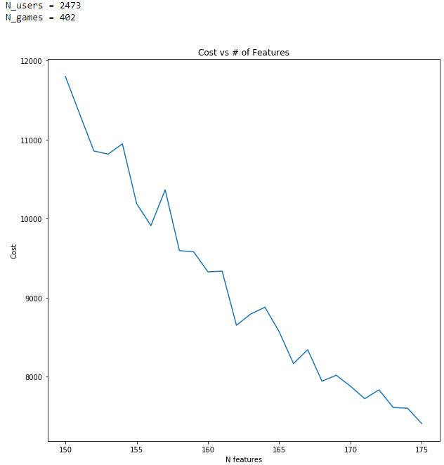
Figure 3 shows the model’s error dependence on the number of features, N. As the number of features increases, the model’s error decreases. This is exactly what one should expect. If we attempt to predict user ratings of games given only the recommended age of the games, you can imagine the results would be quit unreliable. If however, we are given the game’s recommended age, genre, number of players, game length, etc., the results should be more accurate.

Figure 4 | Training Results

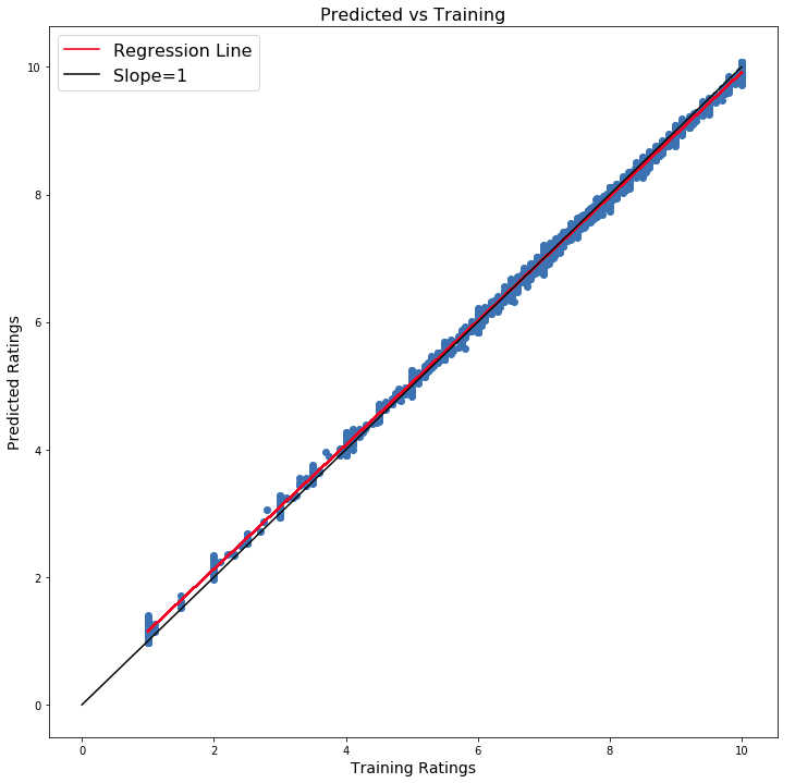
Figure 4 shows the results of training the model. The predicted ratings are plotted against the actual ratings in the training data set. This gives a visual indication of how well the model fits the data based on the spread of points from the line with slope unity. If the model predicts the ratings perfectly, the points will all lie exactly on the black line. Of course, such a model would likely be prone to overfitting so including a regularization term can help mitigate overfitting.

Figure 5 | Prediction Results

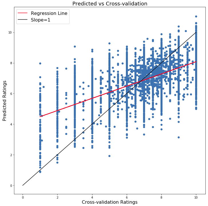
After training the model, we can make predictions on the CV data set. Figure 5 shows the predicted ratings vs the actual ratings in the CV data set. The red line shows the line of best fit for the data. We can see the best fit line is quite skewed compared to the line with slope unity. The model tends to predict higher than the actual values at lower ratings while it tends to under predict at higher ratings. The regression line crosses the ideal line at around the median total rating. Also notice that at the higher ratings, some predictions are actually above 10 (10 is the maximum rating possible). This is something we can easily fix by setting boundaries on the model’s output.

Summary

In this part of the recommender system series, I demonstrated how to build a collaborative filtering model for predicting user ratings of board games. The model is able to fit the training data well but shows room for improvement in predictions on the cross-validation data. In the next part of this series, I will explore methods for optimizing this model so that it can generalize better to the cross-validation data.