
Race & Sex Discrimination in US Job Market
Background
Race & sex discrimination is still a topic of interest in today’s job market. To examine discrimination in these two categories, Bertrand, Marianne, and Sendhil Mullainathan created a blind study. Fictitious resumes, 50% with white-sounding names and 50% with black-sounding names, were randomly sent to job postings in the Boston & Chicago newspapers. Here I will employ statistical tests to determine if there is a statistically significant difference between the number of callbacks that black-sounding vs white-sounding and male vs female populations get.
For the original paper and dataset, see study cited below.
CITATION: Bertrand, Marianne, and Sendhil Mullainathan. 2004. “Are Emily and Greg More Employable Than Lakisha and Jamal? A Field Experiment on Labor Market Discrimination.” American Economic Review, 94 (4): 991-1013.
DOI: 10.1257/0002828042002561
Hypotheses
The null and alternate hypotheses in both cases of race and sex are similar. The null hypothesis is that the difference in proportion of callbacks between the two populations is equal to 0, or there is no difference. While the alternative hypothesis is that the difference in proportion of callbacks between the two populations is not equal to 0, in which case there is a difference. Mathematically, the hypotheses can be written as follows:
Race Hypotheses
\[H_0: \bar p_{white} - \bar p_{black} = 0\] \[H_A: \bar p_{white} - \bar p_{black} \neq 0\]Sex Hypotheses
\[H_0: \bar p_{male} - \bar p_{female} = 0\] \[H_A: \bar p_{male} - \bar p_{female} \neq 0\]For the two sets of hypotheses I will use both a frequentist and bootstrap approach and compare these results against each other. In the frequentist approach, I will perform a two-sample t test to compare the means of the two sample populations of interest. This will tell us if the two sample populations belong to the same overall population, that is, their distributions are equal. If their distributions are equal, we have evidence supporting the null hypotheses.
Exploratory Analysis
import pandas as pd
import numpy as np
from scipy import stats
import plotly.graph_objs as go
from plotly.offline import download_plotlyjs, init_notebook_mode, plot, iplot
import plotly.figure_factory as ff

init_notebook_mode(connected=True)
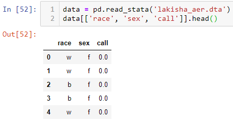
In this study, I will only be using 3 columns from the full dataset. The race, sex, and callback columns which are all binary.
data = pd.read_stata('lakisha_aer.dta')
data[['race', 'sex', 'call']].head()
Table 1 | Sample of Data
# subset the race data into individual dataframes
# 'w' corresponds to white-sounding names
# 'b' corresponds to black-sounding names
w = data[data.race=='w']
b = data[data.race=='b']

# subset the sex data into individual dataframes
# 'm' corresponds to males
# 'f' corresponds to females
m = data[data.sex=='m']
f = data[data.sex=='f']
| Black Sample Size: 2435 | White Sample Size: 2435 |
| Male Sample Size: 1124 | Female Sample Size: 3746 |
We can see that the black and white sample sizes are equal, but this is not true for the male and female sample populations. However, we will avoid issues with unequal sample sizes by using proportions in our analysis.
# visualize the two normalized distributions
trace0 = go.Histogram(x=w.call, name='white', histnorm='probability',
                      marker=dict(color='#FEBC38'))
trace1 = go.Histogram(x=b.call, name='black', histnorm='probability',
                      marker=dict(color='#37AFA9'))

layout = go.Layout(title='Callback Proportions Between Black & White Populations',
                  xaxis=dict(title='Callback (0 if no, 1 if yes)'),
                  yaxis=dict(title='Callback proportion'))

data = [trace0, trace1]

fig = go.Figure(data, layout)

iplot(fig, filename='callback-proportions-black-white.html')
Figure 1 | Callback Proportions Between Black & White Populations
The histogram above shows a small difference between the proportion of callbacks in the black and white sample populations. Specifically, white-sounding names received a callback 9.65% of the time while black-sounding names received a callback only 6.45% of the time. We will find out if this difference is statistically significant.
# visualize the two normalized distributions
trace0 = go.Histogram(x=m.call, name='male', histnorm='probability',
                      marker=dict(color='#B42F32'))
trace1 = go.Histogram(x=f.call, name='female', histnorm='probability',
                      marker=dict(color='#27647B'))

layout = go.Layout(title='Callback Proportions Between Male & Female Populations',
                  xaxis=dict(title='Callback (0 if no, 1 if yes)'),
                  yaxis=dict(title='Callback proportion'))

data = [trace0, trace1]

fig = go.Figure(data, layout)

iplot(fig, filename='callback-proportions-male-female.html')
Figure 2 | Callback Proportions Between Male & Female Populations
The difference in proportion of callbacks is much smaller between the male (7.38%) and female (8.25%) sample populations. Again, we’ll determine if this difference is statistically significant using our hypothesis testing.
Hypothesis Testing
Frequentist Approach
For the frequentist approach we can conduct a two-sample t-test for the difference of means of the two samples. In this case, the mean of each sample is equal to the proportion of callbacks. This is equivalent to testing whether the white and black samples come from the same distribution (null hypothesis), or they come from two different distributions (alternate hypothesis).
I’m interested in testing my hypothesis at the 95% confidence level. This corresponds to a critical value of alpha=0.05. Now I can compute the two-sample t-statstic for the difference of means of my two samples.
# of samples n is equal for both black and white sample populations
n = len(w.call)

# compute means
w_mean = np.mean(w.call)
b_mean = np.mean(b.call)

# compute standard deviations
w_std = np.std(w.call)
b_std = np.std(b.call)

print('Black mean: %s' % round(b_mean, 4))
print('White mean: %s' % round(w_mean, 4))
print('Black std: %s' % round(b_std, 4))
print('White std: %s' % round(w_std, 4))
| Black mean: 0.0645 | White mean: 0.0965 |
| Black std: 0.2456 | White std: 0.2953 |
# compute the standard error
SE = np.sqrt((w_std**2)/n + (b_std**2)/n)

# compute the t-statistic
t = (w_mean - b_mean)/SE
print('t stat: %s' % round(t, 3))

# compute degrees of freedom
DF = n - 1

# compute the p-value associated with the t-stat
p_value = stats.t.sf(t, DF)*2
print('p-value: %s' % round(p_value, 6))
The t-statistic I get is 4.116 which corresponds to a p-value of 0.00004. This is much less than my critical value of alpha=0.05. Therefore I can say with 95% confidence that the null hypothesis can be rejected, suggesting the alternative hypothesis that the proportion of white resumes receiving a callback is NOT equal to the proportion of black resumes receiving a callback.
# difference in sample means
diff = round(w_mean - b_mean, 3)

# t-value corresponding to 95% CI
t_star = 1.96

# calculate upper and lower CI
lower_CI = round(diff - t_star*SE, 3)
upper_CI = round(diff + t_star*SE, 3)

print(f"The difference in proportion of callbacks between black and \
white populations is {diff} with a lower 95% CI of {lower_CI} and \
an upper 95% CI of {upper_CI}")
Since we have support for the alternate hypothesis, we can calculate the difference between the two proportions and the 95% confidence intervals. The difference in proportion of callbacks between black and white populations is 0.032 with a lower 95% CI of 0.017 and an upper 95% CI of 0.047.
We follow the same calculations for the male and female sample populations.
# in this case, we use the smaller of the sample sizes.
n = len(m.call)

# compute means
m_mean = np.mean(m.call)
f_mean = np.mean(f.call)

# compute standard deviations
m_std = np.std(m.call)
f_std = np.std(f.call)

# compute the standard error
SE = np.sqrt((m_std**2)/n + (f_std**2)/n)

# compute the t-statistic
t = (f_mean - m_mean)/SE

# compute degrees of freedom
DF = n - 1

# compute the p-value associated with the t-stat
p_value = stats.t.sf(t, DF)*2

print('p-value: %s' % round(p_value, 3))
For the male vs female populations, the p-value comes out to 0.445. This is much larger than 0.05 so we cannot reject the null hypothesis.
Using the frequentist approach we can conclude that there is a statistically significant difference between the proportion of black-sounding and white-sounding names in resumes that receive a callback for an interview, with white-sounding names having a higher proportion of callbacks.
However, we found no statistically significant evidence that there is a difference in proportion of callbacks between male and female sample populations.
Bootstrapping approach
This problem can be modeled as a Bernoulli trial because:
Each trial is assumed to be independent. Whether or not a resume receives a callback does not depend on whether any of the other resumes in the experiment received a callback or not. Each trial has a pass/fail outcome (1 if the resume received a callback and 0 if not). We can thus model the two resume samples using np.random.binomial, take the difference of their means (proportion of callbacks) and create a bootstrap population of the difference of means. Then we can use a Z test to test the null and alternate hypotheses.
The function below creates two bootstrap samples, computes the difference in their means (proportion of callbacks), stores the difference in p_bootstrap, and does this n_samples times.
def create_bootstrap_sample(sample1_mean=None, sample2_mean=None,
                            sample_size=100, n_samples=1000,
                            random_seed=None):
    if random_seed != None:
        # Seed random number generator
        np.random.seed(random_seed)
    """Create a bootstrap sample population of the difference of
    proportions between sample1 and sample2 populations."""

    # create an empty array to store the difference in proportions
    # from each bootstrap sample
    p_bootstrap = np.empty(n_samples)

    for i in range(0,n_samples):
        # sample proportion of sample1
        sample1_p = np.random.binomial(sample_size, sample1_mean, size=1)/sample_size
        # sample proportion of sample2
        sample2_p = np.random.binomial(sample_size, sample2_mean, size=1)/sample_size

        diff = sample2_p - sample1_p

        # store the difference of proportions
        p_bootstrap[i] = diff

    return p_bootstrap
# create the bootstrap sample population using the above function
p_bootstrap_race = create_bootstrap_sample(sample1_mean=b.call.mean(), sample2_mean=w.call.mean(),
                                      sample_size=n, n_samples=5000, random_seed=42)

print('Race Bootstrap population mean: %s' % round(np.mean(p_bootstrap_race), 4))
print('Race Bootstrap population std: %s' % round(np.std(p_bootstrap_race), 4))
Race Bootstrap population mean: 0.032 Race Bootstrap population std: 0.0115
It’s important to note that the sample size of each bootstrap sample must be the same as the original black and white sample populations so as to not affect the variance of the bootstrap sample population. Since a higher sample size will lead to a lower standard deviation. The number of bootstrap samples we create however will not affect the individual bootstrap population variance.
# visualize the two normalized distributions
trace0 = go.Histogram(x=p_bootstrap_race, name='race',
                      marker=dict(color='#37AFA9'))

layout = go.Layout(title='Bootstrap Sample Differences - Race',
                  xaxis=dict(title='Difference in Proportion'),
                  yaxis=dict(title='Count'))

data = [trace0]

fig = go.Figure(data, layout)

iplot(fig, filename='bootstrap-distribution-race.html')
Figure 3 | Bootstrap Sample Differences - Race
The plot above shows the distribution of all the differences calculated between the black and white bootstrap sample populations. We can see it’s centered around 0.032 and falls off quickly at around 0.01 and 0.05.
# create the bootstrap sample population using the above function
p_bootstrap_sex = create_bootstrap_sample(sample1_mean=m.call.mean(), sample2_mean=w.call.mean(),
                                      sample_size=n, n_samples=5000, random_seed=42)

# visualize the two normalized distributions
trace0 = go.Histogram(x=p_bootstrap_sex, name='race',
                      marker=dict(color='#B42F32'))

layout = go.Layout(title='Bootstrap Sample Differences - Sex',
                  xaxis=dict(title='Difference in Proportion'),
                  yaxis=dict(title='Count'))

data = [trace0]

fig = go.Figure(data, layout)

iplot(fig, filename='bootstrap-distribution-sex.html')
Figure 4 | Bootstrap Sample Differences - Sex
Using the same function to generate bootstrap samples for the male and female sample populations, we get the distribution above. The mean is closer to 0.023 and the lower tail shows negative differences. Implying that in some of the bootstrap samples generated, the proportion of males receiving callbacks is actually higher than the proportion of females receiving callbacks.
We can get a better idea of our test result by visualizing the Empirical Cumulative Distribution Function (ECDF) of the bootstrap sample populations.
def ecdf(data):
    """Compute ECDF for a one-dimensional array of measurements."""
    # Number of data points: n
    n = len(data)

    # x-data for the ECDF: x
    x = np.sort(data)

    # y-data for the ECDF: y
    y = np.arange(1, len(data) + 1) / n

    return x, y
# compute the ecdf for both distributions
x_race, y_race = ecdf(p_bootstrap_race)
x_sex, y_sex = ecdf(p_bootstrap_sex)

# plot the two ecdfs
trace0 = go.Scattergl(x=x_race, y=y_race, mode='markers', name='Race')
trace1 = go.Scattergl(x=x_sex, y=y_sex, mode='markers', name='Sex')

layout = go.Layout(title='ECDF of Bootstrap Sample Differences',
                  xaxis=dict(title='Difference in Proportion'),
                  yaxis=dict(title='Probability'))

data = [trace0, trace1]

fig = go.Figure(data, layout)

iplot(fig, filename='ecdf-race-sex.html')
Figure 5 | ECDF of Bootstrap Sample Differences
Comparing the two ECDFs above, we can see that the distribution of differences in proportions of callbacks for sex sits further to the left than for race. The probability of getting a difference in proportion between the black and white sample populations equal to 0 is only 0.2%. While between male and females this probability is equal to 2.5%, more than an order of magnitude higher. This tells us that it is much less likely that the proportion of callbacks is equal between the black and white populations than between males and females.
Now we can calculate the z-score for these two populations and a p-value. I’ll use the same confidence level as in the frequentist approach of 95%, with a corresponding alpha value of 0.05 for the z test.
# define alpha for the 95% confidence interval
alpha = 0.05

# this corresponds to a critical z-score of
z_crit = -1.96
Since we are interested in testing the null hypothesis that the difference in means (proportions) of the two sample populations is equal to zero, we use the value 0, the bootsrap sample population mean and standard deviation to compute a z-score.
# calculate z-score for race bootstrap population
z_race = (0-np.mean(p_bootstrap_race))/np.std(p_bootstrap_race)

print('Z-score - Race: %s' % round(z_race, 2))
print('Critical Z: %s' % z_crit)
| Z-score - Race: -2.79 | Critical Z: -1.96 |
# calculate z-score for sex bootstrap population
z_sex = (0-np.mean(p_bootstrap_sex))/np.std(p_bootstrap_sex)

print('Z-score - Sex: %s' % round(z_sex, 2))
print('Critical Z: %s' % z_crit)
| Z-score - Sex: -1.91 | Critical Z: -1.96 |
Regarding the black and white populations, the z-score of -2.79 is much less than the critical Z of -2.33. The z-score of -2.79 corresponds to a p-value of 0.00527, which is again much less than the 0.05. Thus we reach the same conclusion as in the frequentist approach and can reject the null hypothesis in support of the alternate hypothesis.
For the male vs female populations, the z-score is -1.91 which is just larger than our critical z-score of -1.96. The associated p-value is 0.056, which is not significant. Therefore, we cannot reject the null hypothesis and thus cannot say that the proportion of callbacks between males and females are different.
Conclusions
In both the frequentist and bootstrapping approaches, I found with 95% confidence and statistical significance, evidence to reject the null hypothesis and accept the alternate hypothesis that the porportion of “black” resumes that receive callbacks is NOT equal to the proportion of “white” resumes that receive callbacks. The same cannot be said between male and female populations.
The results of my analysis does not imply that race/name is the most important factor in callback success. The result only implies that there is a difference in callback success between two populations (black and white). There may in fact be other underlying factors that drive callback success which were not tested for here. For example, the level of education could be more important.
To test for these other factors, I would have to perform the analysis comparing the proportions of callbacks for the two populations of each factor I was interested in. For example, I could perform the same tests for the two populations where one has candidates that have higher education and one where candidates had at most a bachelors. I could do this for each of the factors I was interested in, determine which ones were statistically significantly different, and take the one with the largest difference in proportions of callback success as the most important factor.


Leave a Comment